Negative Power Functions

Overview

Now that we have considered the quantum linear system problem (QLSP), it is natural to consider the following generalization: given access to an invertible matrix A and a normalized quantum state \(|b\rangle\), we want to construct a quantum state

\[|x\rangle := \frac{A^{-c} |b\rangle}{\| A^{-c} |b\rangle \|_2},\]

where \(c\) is an integer larger than 1. The implementation boils down to a scalar function \(f(x) = x^{-c}\). Without loss of generality, we assume the matrix is normalized. As before, we want a polynomial with parity approximating \(f(x)\) over the interval \(D_\kappa := [-1,-\kappa] \cup [-\kappa,1]\).

Setup

Just as with QLSP, we will let \(\kappa = 10\) and scale the target function for numerical stability. For \(c = 2\), we can use the scaling factor \(1/(2\kappa^c)\), i.e.,

\[f(x)=\frac{1}{2(\kappa x)^c}, \quad \max_{x \in D_\kappa} |f(x)| = \frac{1}{2}.\]

import numpy as np

kappa = 10
targ = lambda x: 1/(x**2)
deg = 150
parity = deg % 2

opts = {
    'intervals': [1/kappa, 1],
    'objnorm': np.inf,
    'epsil': 0.2,
    'npts': 400,
    'fscale': 1/(2*kappa**2),
    'isplot': True,
    'method': 'cvxpy'
}

Polynomial approximation

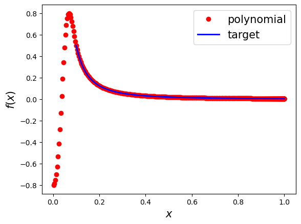
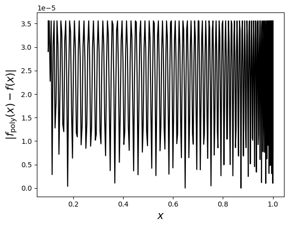
As before, we want to find the best approximation polynomial with degree up to \(d\) in terms of the \(L_\infty\) norm. We call cvx_poly_coef with the above opts to solve the optimization problem and output the Chebyshev coefficients of the best approximation polynomial. Once again, the solver outputs all coefficients while we have to post-select those of odd order due to the parity constraint.

from qsppack.utils import cvx_poly_coef

coef_full = cvx_poly_coef(targ, deg, opts)
coef = coef_full[parity::2]

norm error = 3.5569099550603056e-05
max of solution = 0.7999999443448723

Solving the phase factors and verifying

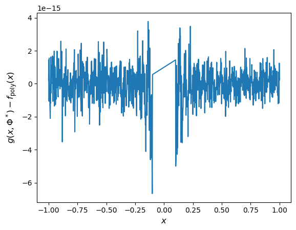
We can again use Newton’s method to find the phase factors and verify the solution.

opts.update({
    'maxiter': 100,
    'criteria': 1e-14,
    'useReal': False,
    'targetPre': True,
    'method': 'Newton'
})

from qsppack.solver import solve
phi_proc, out = solve(coef, parity, opts)

from qsppack.utils import chebyshev_to_func, get_entry
import matplotlib.pyplot as plt

xlist1 = np.linspace(-1,-1/kappa,500)
xlist2 = np.linspace(1/kappa,1,500)
xlist = np.concatenate([xlist1, xlist2])
func = lambda x: chebyshev_to_func(x, coef, parity, True)
targ_value = targ(xlist)
func_value = func(xlist)
QSP_value = get_entry(xlist, phi_proc, out)
err = np.linalg.norm(QSP_value - func_value, np.inf)
print('The residual error is')
print(err)

plt.plot(xlist, QSP_value - func_value)
plt.xlabel('$x$', fontsize=12)
plt.ylabel('$g(x,\\Phi^*)-f_\\mathrm{poly}(x)$', fontsize=12)
plt.show()

iter err
   1  +1.4304e-01
   2  +1.0329e-02
   3  +8.1428e-05
   4  +5.3832e-09
Stop criteria satisfied.
The residual error is
6.661338147750939e-15

Reference

1. Gilyén, A., Su, Y., Low, G. H., & Wiebe, N. (2019, June). Quantum singular value transformation and beyond: exponential improvements for quantum matrix arithmetics. In Proceedings of the 51st Annual ACM SIGACT Symposium on Theory of Computing (pp. 193-204).

2. Dong, Y., Meng, X., Whaley, K. B., & Lin, L. (2021). Efficient phase-factor evaluation in quantum signal processing. Physical Review A, 103(4), 042419.