Hamiltonian Simulation

Overview

The goal in Hamiltonian simulation problems is to implement the map \(H \mapsto \text{exp}(-i\tau H)\) for some Hermitian matrix \(H\) (the Hamiltonian). Using QSP, we can reduce this problem to setting our target scalar function to \(f(x) = \text{exp}(-i\tau x)\). Due to our parity constraint, the implementation of the target scalar function is separated into implementing components \(f_{\text{Re}}(x) = \cos(\tau x)\) and \(f_{\text{Im}}(x) = \sin(\tau x)\) respectively. These components can then be combined to realize \(\text{exp}(-i\tau H)\) using linear combination of unitaries (LCU). To illustrate this workflow, we will choose \(\tau = 100\).

tau = 100

opts = {
    'maxiter': 100,
    'criteria': 1e-12,
    'useReal': True,
    'method': 'Newton' # MATLAB QSPPACK tutorial uses CM
}

Solving for the real component

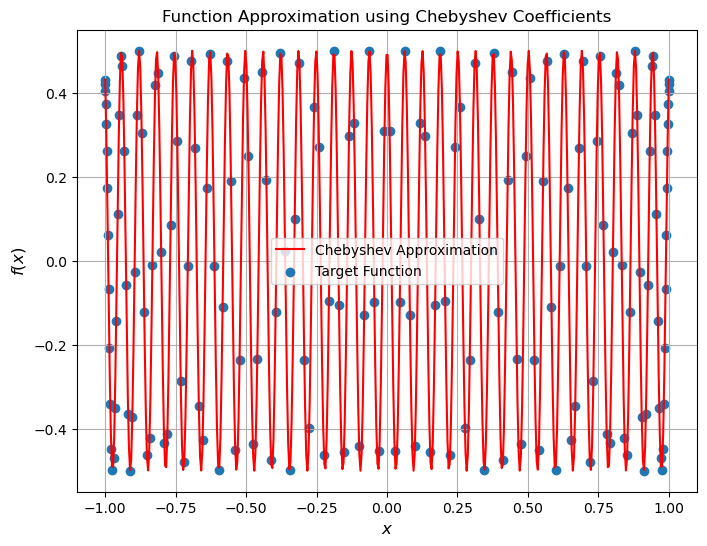
To increase the numerical stability, the real component of the target function is scaled down by a factor of \(\frac{1}{2}\). This scaling causes the target function to be uniformly upper bounded by \(\frac{1}{2}\). The Chebyshev coefficients of the target function are obtained by truncating the series to some finite degree, where it suffices to set \(d=1.4|\tau|+\log\left( \frac{1}{\epsilon_0}\right)\) so that the truncation error is below \(\epsilon_0\).

import numpy as np
from numpy.polynomial.chebyshev import chebinterpolate

# Define the target function
def targ(x):
    return 0.5 * np.cos(tau * x)

# Compute the degree for Chebyshev approximation
d = int(np.ceil(1.4 * tau + np.log(1e14)))+1
parity = d % 2

# Generate Chebyshev coefficients
xpts = np.cos(np.pi * (np.arange(d)+0.5) / d)
f_values = targ(xpts)
coef = chebinterpolate(targ, d)

# Discard coefficients of odd orders due to the even parity
print(f"Should be 0 due to even parity:\t{max(coef[parity+1::2])}")
coef_even = coef[parity::2]

Should be 0 due to even parity: 2.0301221021717148e-17

import matplotlib.pyplot as plt
from numpy.polynomial.chebyshev import chebval

# Define a range of x values for plotting
x_values = np.linspace(-1, 1, 500)

# Evaluate the Chebyshev polynomial at these x values
y_values = chebval(x_values, coef)

# Plot the function
plt.figure(figsize=(8, 6))
plt.plot(x_values, y_values, label='Chebyshev Approximation', color="red")
plt.scatter(xpts, f_values, label='Target Function')
plt.xlabel('$x$', fontsize=12)
plt.ylabel('$f(x)$', fontsize=12)
plt.title('Function Approximation using Chebyshev Coefficients')
plt.legend()
plt.grid(True)
plt.show()

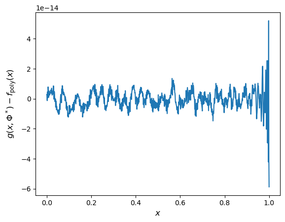
Solving the phase factors and verifying

We can again use Newton’s method to find the phase factors and verify the solution.

from qsppack.solver import solve
phi_proc, out = solve(coef_even, parity, opts)

from qsppack.utils import chebyshev_to_func, get_entry
import matplotlib.pyplot as plt

xlist = np.linspace(0, 1, 1000)
targ_value = targ(xlist)
QSP_value = get_entry(xlist, phi_proc, out)
err = np.linalg.norm(QSP_value - targ_value, np.inf)
print('The residual error is')
print(err)

plt.plot(xlist, QSP_value - targ_value)
plt.xlabel('$x$', fontsize=12)
plt.ylabel('$g(x,\\Phi^*)-f_\\mathrm{poly}(x)$', fontsize=12)
plt.show()

iter err
   1  +1.7869e-01
   2  +1.8346e-03
   3  +1.4232e-07
Stop criteria satisfied.
   3  +1.4232e-07
Stop criteria satisfied.
The residual error is
5.873079800267078e-14
The residual error is
5.873079800267078e-14

Reference

1. Low, G. H., & Chuang, I. L. (2017). Optimal Hamiltonian simulation by quantum signal processing. Physical review letters, 118(1), 010501.

2. Gilyén, A., Su, Y., Low, G. H., & Wiebe, N. (2019, June). Quantum singular value transformation and beyond: exponential improvements for quantum matrix arithmetics. In Proceedings of the 51st Annual ACM SIGACT Symposium on Theory of Computing (pp. 193-204).

3. Dong, Y., Meng, X., Whaley, K. B., & Lin, L. (2021). Efficient phase-factor evaluation in quantum signal processing. Physical Review A, 103(4), 042419.

Additional plots

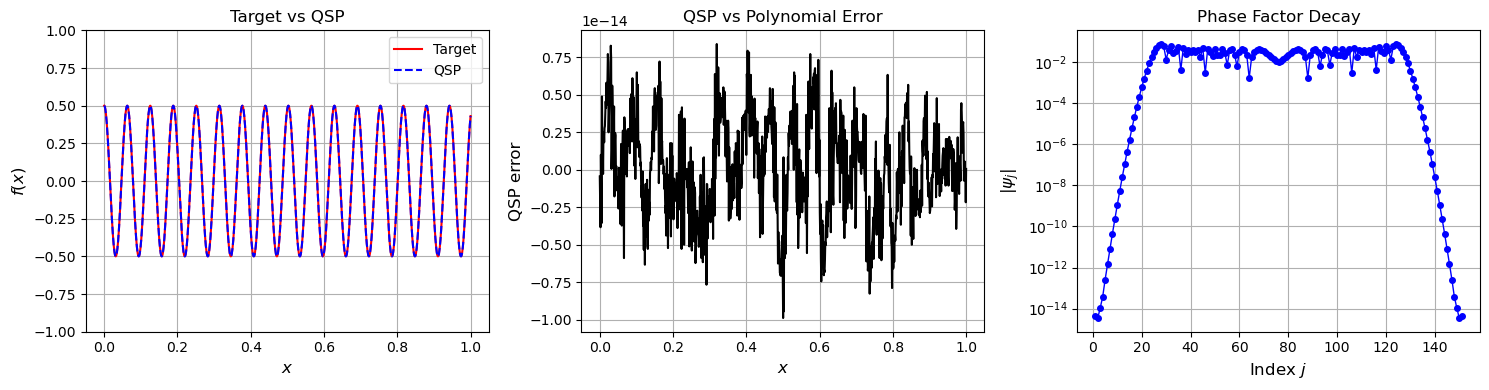
Consider \(f(x)=\frac{1}{2} \cos(100 x)\). We can first approximate \(f(x)\) by an even polynomial \(p(x)\) using Chebyshev interpolation, and then use Newton’s method to find phase factors \(\Psi\) such that \(\Re[U_d(x,\Psi)]_{1,1}=p(x)\).

# Recalculate with higher degree for high-precision example
d_high = 150
parity = 0  # Even parity for cosine function

# Generate Chebyshev coefficients with higher degree
coef_high = chebinterpolate(targ, d_high)

# Extract even coefficients only (due to even parity)
coef_even_high = coef_high[parity::2]

print(f"Degree of the approximating polynomial: {d_high}")
print(f"Number of even coefficients: {len(coef_even_high)}")

# Set up solver options - use Newton method like the working example
opts_high = {
    'maxiter': 100,
    'criteria': 1e-14,
    'useReal': True,
    'method': 'Newton'
}

# Solve for phase factors
phi_proc_high, out_high = solve(coef_even_high, parity, opts_high)

print(f"Converged in {out_high['iter']} iterations")

Degree of the approximating polynomial: 150
Number of even coefficients: 76
iter err
   1  +1.7869e-01
   2  +1.8346e-03
   3  +1.4232e-07
Stop criteria satisfied.
Converged in 4 iterations

# Evaluate the functions for comparison
xlist = np.linspace(0, 1, 1000)
targ_value = targ(xlist)
func_value = chebval(xlist, coef_high)  # Polynomial approximation
QSP_value_high = get_entry(xlist, phi_proc_high, out_high)

# Calculate errors
poly_error = np.linalg.norm(QSP_value_high - func_value, 1) / len(xlist)
qsp_error = np.linalg.norm(QSP_value_high - targ_value, 1) / len(xlist)

print('The QSP vs polynomial error is:', poly_error)
print('The QSP vs target error is:', qsp_error)

# Prepare phase factors with pi/4 removed from both ends
phi_shift = phi_proc_high.copy()
phi_shift[0] = phi_shift[0] - np.pi/4
phi_shift[-1] = phi_shift[-1] - np.pi/4

The QSP vs polynomial error is: 2.5865713040927432e-15
The QSP vs target error is: 5.542973564409519e-15

# Generate the three-subplot figure matching the MATLAB version
fig, axes = plt.subplots(1, 3, figsize=(15, 4))

# Left subplot: polynomial approximation vs actual function
axes[0].plot(xlist, targ_value, 'r-', linewidth=1.5, label='Target')
axes[0].plot(xlist, QSP_value_high, 'b--', linewidth=1.5, label='QSP')
axes[0].set_xlabel('$x$', fontsize=12)
axes[0].set_ylabel('$f(x)$', fontsize=12)
axes[0].set_ylim([-1, 1])
axes[0].legend(loc='best')
axes[0].grid(True)
axes[0].set_title('Target vs QSP')

# Middle subplot: error between QSP and polynomial approximation
axes[1].plot(xlist, QSP_value_high - func_value, 'k-', linewidth=1.5)
axes[1].set_xlabel('$x$', fontsize=12)
axes[1].set_ylabel('QSP error', fontsize=12)
axes[1].grid(True)
axes[1].set_title('QSP vs Polynomial Error')

# Right subplot: phase factors (after removing pi/4 factor) on log scale
axes[2].semilogy(range(1, len(phi_shift)+1), np.abs(phi_shift), 'bo-', markersize=4, linewidth=1)
axes[2].set_xlabel('Index $j$', fontsize=12)
axes[2].set_ylabel('$|\\psi_j|$', fontsize=12)
axes[2].grid(True)
axes[2].set_title('Phase Factor Decay')

plt.tight_layout()
# plt.savefig('qsp_cos100x.png', dpi=300, bbox_inches='tight')
# print(f"Figure saved as 'qsp_cos100x.png'")
plt.show()